Introduction
In this post we’ll be covering Content-based filtering and Collaborative theories. These are traditional recommendation models but are important concepts in recommendation system literature and will help pave the foundation for more advanced models that we’ll be discussing later on.
Let’s delve deep 🔍
So there are many traditional approaches used to build recommendation systems. One common approach is Content-based theory. Content-based filtering uses item features to recommend other items similar to what a user likes based on previous actions or explicit feedback.
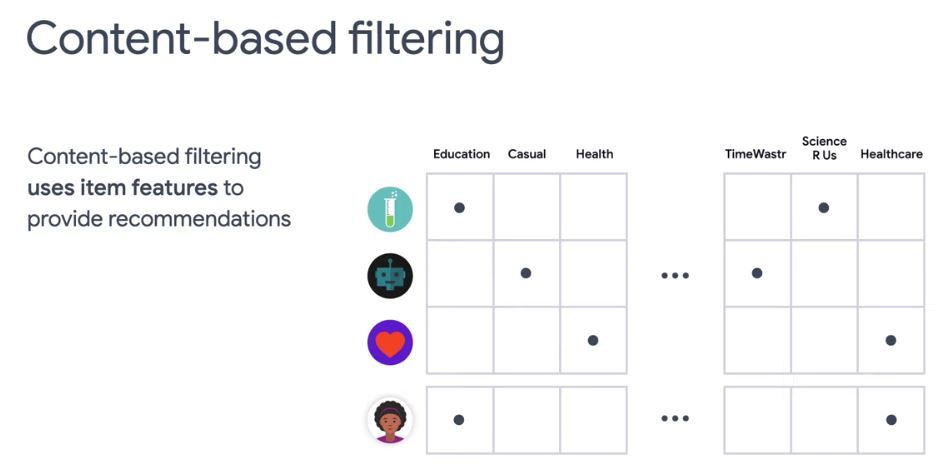
For example here we’re illustrating four apps that have different features. Each row represents an app and each column represents a feature. Some apps are educational or science related, some are relevant to health or healthcare. Some are simply time wasters. When a user installs a health app we can recommend other health related apps to that user because they are similar to the installed health app.
Another common approach is Collaborative filtering. One limitation with content-based filtering is that it only leverages item similarities. Now, what if we can use similarities between users and items simultaneously to provide recommendations, this would allow for serendipitous recommendations namely recommending an item to user A based on the interest of a similar user B. This is what collaborative filtering is able to do, while item-based filtering is not.
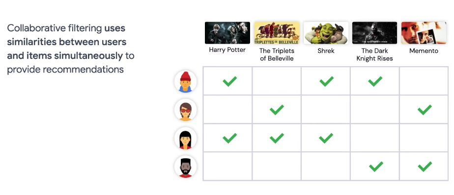
Here we are illustrating a feedback matrix of 4 users and 5 movies. Each row represents a user and each column represents a movie the green check mark means that a user has watched a particular movie. We consider this an implicit feedback. In contrast, if a user gives a rating on the movie, that would be an explicit feedback. So as you can see here, the user in the first row has watched the three movies Harry Potter, Shrek and The Dark Knight Rises.
Now for the user in the third row, she has also watched the Harry Potter and Shrek. So it may make sense to recommend The Dark Knight Rises to her, since the first user has similar preference to her.
💡 So that’s the idea of Collaborative theory!
But how do we do this in practice? 🤔
Let’s say we can assign a value between -1 to 1 to each user indicating their interest level for children’s movies. -1 means highest level of interest for children’s movies and 1 means no interest at all. In this case user number 3 likes children’s movies a lot and user number 4 doesn’t like children’s movies at all.
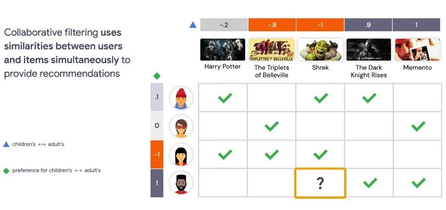
We can also assign a value between -1 to 1 to each movie -1 means the movie is highly suitable for children and 1 means, it’s not for children at all.
Now, we can see Shrek is really a great movie for children. Now these values become embedding for users and movies, and the product of user embedding and moving betting should be higher for movies that we expected the user to like.
In this example, we hand engineered these embeddings and these embeddings are one-dimensional.
Now, we can say, we have another dimension to represent the users in the movies. Let’s assign another value between -1 to 1 to each user, indicating their interest level for blockbuster movies. Similarly, we assign a value between -1 to 1 to each movie, indicating whether it is blockbuster or not.
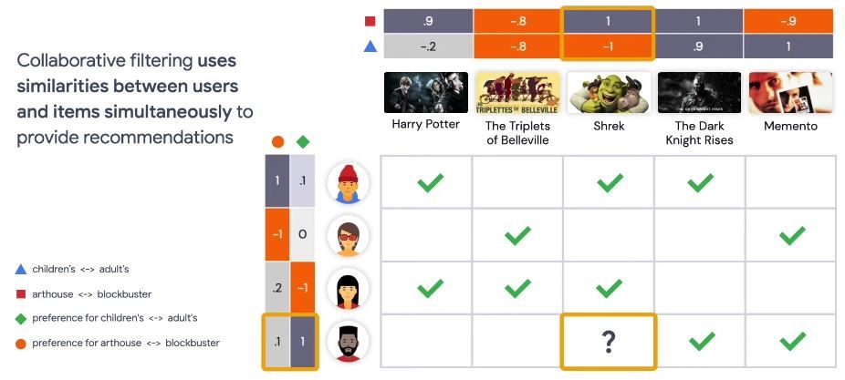
Now we have hand engineered the second dimension of embeddings. We can go on and add more dimensions if we want.
In practice these embeddings tend to be of much higher dimensions, but we can learn those embeddings automatically, which is the real beauty of Collaborative filtering models.
For the sake of easier visualization, we are sticking to two dimensions (2D). Here, we are illustrating 2D embeddings for the users and movies on the right.
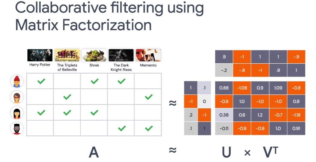
Our goal is to make sure that we can learn this embeddings so that the predictive feedback matrix is as close to the ground truth feedback matrix as possible.
Here, we denote user embeddings at U and item embeddings at V. The product of U and V is A, which is a predicted feedback matrix.
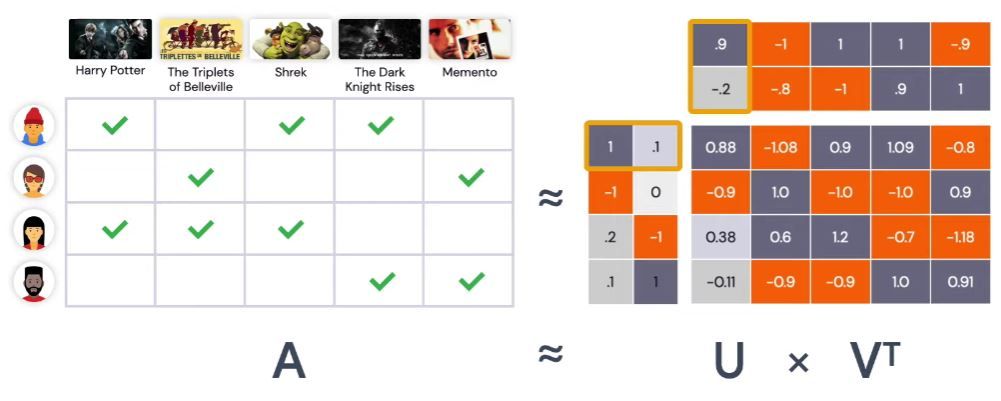
For example, if we take the first row of U, 1, 0.1, and the first column of V, 0.9, 0.2, and compute the dot product it gives 0.88, which is the top left-most element in the predict feedback matrix.
So, our optimization objective then becomes minimizing the summation of the squared difference between the feedback label and the predictive feedback!
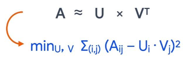
As you can see in the mathematical form in blue we can solve this using either Stochastic Gradient Descent (SGD) or Weighted Alternating List Squares (WALS). SGD is a very pronounced concept in terms of Neural Networks. SGD is a generic message, while WALS is specific to this problem.
The idea of WALS is that, for each iteration we alternate between fixing U and solve for V and then fixing V and solving for U.
We won’t go into the mathematical details, but I should point out that SGD and WALS each have their own advantages and disadvantages. For example WALS usually converges much faster than sgd, while sgd is more flexible and can handle other loss functions.
But so far, we only cared about observed items. What about the unobserved ones?
So observed, only matrix factorization is not good! Because if you set the embeddings to all 1’s, you have minimized the objective function, which is clearly not we want. So we need to take into account of the unobserved entries. There are two approaches to handle thi. First we can treat all unobserved entries as 0, and then solve it using SVD — Singular Value Decomposition. We won’t be reviewing linear algebra here, but you should know that SVD is not very good at this, because the A matrix tends to be very sparse in practice. So, the SVD solution tends to have poor generalization capabilities.
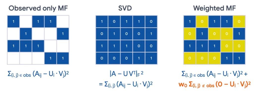
A better approach is Weighted Matrix Factorization. In this case, we still treat unobserved entries as zero, but we scale the unobserved part of the object function, highlighted in orange, so that it’s not overweighted. As you can see the weight w0 is now a hyperparameter you need to tune.
References
- Recommnedation systems on Google Developers website → https://developers.google.com/machine-learning/recommendation
- Building a Recommendation system using SGD → https://developers.google.com/machine-learning/recommendation/labs/movie-rec-programming-exercise
- Building a Recommendation model using WALS on Google Cloud → https://developers.google.com/machine-learning/recommendation
- Neural Collaborative Filtering implementation in TensorFlow Model Garden → https://goo.gle/3qSrEBg
That is all, I hope you liked the post. Thank you very much for reading, and have a great day! 😄