The Beginning
In the beginning, learning Machine Learning (ML) can be intimidating. Terms like “Gradient Descent”, “Latent Dirichlet Allocation” or “Convolutional Layer” can scare lots of people 🤯. But there are friendly ways of getting into the discipline, and I think starting with Decision Trees is a wise decision.
Decision Trees (DTs) are probably one of the most useful supervised learning algorithms out there. As opposed to unsupervised learning (where there is no output variable to guide the learning process and data is explored by algorithms to find patterns), in supervised learning your existing data is already labelled and you know which behaviour you want to predict in the new data you obtain. This is the type of algorithms that autonomous cars use to recognize pedestrians and objects, or organizations exploit to estimate customers lifetime value and their churn rates.
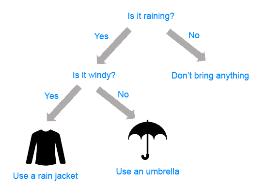
❝In a way, supervised learning is like learning with a teacher, and then apply that knowledge to new data.❞
DTs are ML algorithms that progressively divide data sets into smaller data groups based on a descriptive feature, until they reach sets that are small enough to be described by some label. They require that you have data that is labelled (tagged with one or more labels, like the plant name in pictures of plants), so they try to label new data based on that knowledge.
So, where do we use it?
DTs algorithms are perfect to solve classification (where machines sort data into classes, like whether an email is spam or not) and regression (where machines predict values, like a property price) problems. Regression Trees are used when the dependent variable is continuous or quantitative (e.g. if we want to estimate the probability that a customer will default on a loan), and Classification Trees are used when the dependent variable is categorical or qualitative (e.g. if we want to estimate the blood type of a person).
The importance of DTs relies on the fact that they have lots of applications in the real world. Being one of the mostly used algorithms in ML, they are applied to different functionalities in several industries:
DTs are being used in the healthcare industry to improve the screening of positive cases in the early detection of cognitive impairment, and also to identify the main risk factors of developing some type of dementia in the future.
Sophia, the robot that was made a citizen of Saudi Arabia, uses DTs algorithms to chat with humans. In fact, chatbots that use these algorithms are already bringing benefits in industries like health insurance by gathering data from customers through the application of innovative surveys and friendly chats. Google recently acquired Onward, a company that uses DTs to develop chatbots that are exceptionally functional in delivering world-class customer care, and Amazon is investing in the same direction to guide customers quickly to a path of resolution.
It is possible to predict the most likely causes of forest disturbances, like wildfire, logging of tree plantations, large or small scale agriculture, and urbanization by training DTs to recognize different causes of forest loss from satellite imagery. DTs and satellite imagery are also used in agriculture to classify different crop types and identify their phenological stages.
DTs are great tools to perform sentiment analysis of texts, and identify the emotions behind them. Sentiment analysis is a powerful technique that can help organizations to learn about customers choices and their decision drivers.
DTs are also used to improve financial fraud detection. The MIT showed that it could significantly improve the performance of alternative ML models by using DTs that were trained with several sources of raw data to find patterns of transactions and credit cards that match cases of fraud.
DTs are extremely popular for a variety of reasons, being their interpretability probably their most important advantage. They can be trained very fast and are easy to understand, which opens their possibilities to frontiers far beyond scientific walls. Nowadays, DTs are very popular in business environments and their usage is also expanding to civil areas, where some applications are raising big concerns.
Tree-based methods can be used for regression or classification. They involve segmenting the prediction space into a number of simple regions. The set of splitting rules can be summarized in a tree, hence the name decision tree methods. A single decision tree is often not as performant as linear regression, logistic regression, LDA, etc. However, by introducing random forests it can result in dramatic improvements in prediction accuracy at the expense of some loss in interpretation.
The Basics
DTs are composed of nodes, branches and leafs. Each node represents an attribute (or feature), each branch represents a rule (or decision), and each leaf represents an outcome. The depth of a Tree is defined by the number of levels, not including the root node.

As previously mentioned, DTs apply a top-down approach to data, so that given a data set, they try to group and label observations that are similar between them, and look for the best rules that split the observations that are dissimilar between them until they reach certain degree of similarity.
❝They use a layered splitting process, where at each layer they try to split the data into two or more groups, so that data that fall into the same group are most similar to each other (homogeneity), and groups are as different as possible from each other (heterogeneity).❞
The splitting can be binary (which splits each node into at most two sub-groups, and tries to find the optimal partitioning), or multiway (which splits each node into multiple sub-groups, using as many partitions as existing distinct values). In practice, it is usual to see DTs with binary splits, but it’s important to know that multiway splitting has some advantages. Multiway splits exhaust all information in a nominal attribute, which means that an attribute rarely appears more than once in any path from the root to the leaf, which make DTs easier to comprehend. In fact, it could happen that the best way to split data might be to find a set of intervals for a given feature, and then split that data up into several groups based on those intervals.
Each feature of the data set becomes a root[parent] node, and the leaf[child] nodes represent the outcomes. The decision on which feature to split on is made based on resultant entropy reduction or information gain from the split.
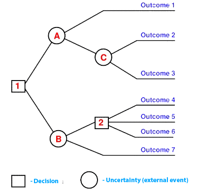
Classification problems for decision trees are often binary — True or False, Male or Female. However, decision trees can also be used to solve multi-class classification problems where the labels are [0, …, K-1], or for this example, [‘Converted customer’, ‘Would like more benefits’, ‘Converts when they see funny ads’, ‘Won’t ever buy our products’].
Using Continuous Variables to Split Nodes in a Decision Tree
Continuous features are turned to categorical variables (i.e. lesser than or greater than a certain value) before a split at the root node. Because there could be infinite boundaries for a continuous variable, the choice is made depending on which boundary will result in the most information gain.
Advantages of Decision Trees
- Decision trees are easy to interpret. While other machine Learning models are close to black boxes, decision trees provide a graphical and intuitive way to understand what our algorithm does.
- To build a decision tree requires little data preparation from the user- there is no need to normalize data.
- Compared to other Machine Learning algorithms Decision Trees require less data to train.
- They can be used for Classification and Regression.
- They are simple.
- They are tolerant to missing values.
Disadvantages of Decision Trees
- Decision trees are prone to overfit noisy data. The probability of overfitting on noise increases as a tree gets deeper.
- They are weak learners. Since a single decision tree normally does not make great predictions, so multiple trees are often combined to make ‘forests’ to give birth to stronger ensemble models.
Random Forest
A bag of decision trees that uses subspace sampling is referred to as a random forest. Only a selection of the features is considered at each node split which decorrelates the trees in the forest. Another advantage of random forests is that they have an in-built validation mechanism. Because only a percentage of the data is used for each model, an out-of-bag error of the model’s performance can be calculated using the 37% of the sample left out of each model.
TensorFlow Open Sources TensorFlow Decision Forests (TF-DF). TF-DF is a collection of production-ready algorithms for training, serving, and interpreting decision forest models, including random forests and gradient boosted trees. With the flexibility and composability of TensorFlow and Keras, one can now utilize these models for classification, regression, and ranking tasks.
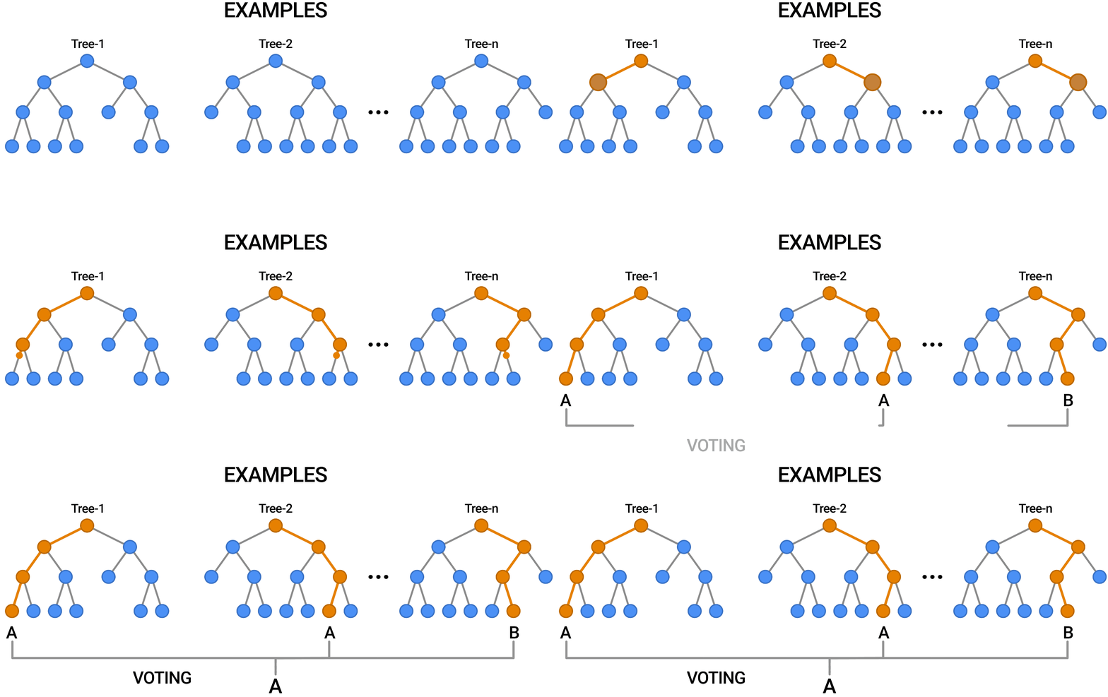
Decision forests are a class of machine learning algorithms that compete with (and frequently outperform) neural networks in quality and performance, especially when working with tabular data. They’re made up of multiple decision trees, making them simple to use and comprehend – and one can utilize a variety of interpretability tools and approaches that are currently available.
The development and explanation of decision forest models will be easier for beginners. There’s no need to list or pre-process input characteristics (decision forests handle numeric and categorical attributes naturally), establish an architecture, or be concerned about models diverging. After your model has been trained, you can plot it or analyze it with simple statistics.
TensorFlow Decision Forests allows you to train state-of-the-art Decision Forests models in TensorFlow with maximum speed, quality, and lowest effort.
Models with a short inference time will help advanced users (sub-microseconds per example in many cases). In addition, this library provides a lot of flexibility for model exploration and research. Combining neural networks and decision forests, in particular, is simple. Random forests, gradient-boosted trees, CART, (Lambda)MART, DART, Extra Trees, greedy global growth, oblique trees, one-side-sampling, categorical-set learning, random categorical learning, out-of-bag evaluation, and feature importance, and structural feature importance are among the state-of-the-art Decision Forest training and serving algorithms available.
By making it easy to connect tree-based models with multiple TensorFlow tools, libraries, and platforms like TFX, this library can serve as a bridge to the rich TensorFlow ecosystem. Users who are new to neural networks can utilize decision forests as an easy method to get started with TensorFlow and then move on to more advanced neural networks.
Training a model
Let’s start with a minimal example where we train a random forest model on the tabular Palmer’s Penguins dataset. The objective is to predict the species of an animal from its characteristics. The dataset contains both numerical and categorical features and is stored as a csv file.

Let’s train a model:
1# Install TensorFlow Decision Forests2!pip install tensorflow_decision_forests34# Load TensorFlow Decision Forests5import tensorflow_decision_forests as tfdf67# Load the training dataset using pandas8import pandas9train_df = pandas.read_csv("penguins_train.csv")1011# Convert the pandas dataframe into a TensorFlow dataset12train_ds = tfdf.keras.pd_dataframe_to_tf_dataset(train_df, label="species")1314# Train the model15model = tfdf.keras.RandomForestModel()16model.fit(train_ds)
Observe that nowhere in the code did we provide input features or hyperparameters. That means, TensorFlow Decision Forests will automatically detect the input features from this dataset and use default values for all hyperparameters.
Evaluating a model
Now, let's evaluate the quality of our model:
1# Load the testing dataset2test_df = pandas.read_csv("penguins_test.csv")34# Convert it to a TensorFlow dataset5test_ds = tfdf.keras.pd_dataframe_to_tf_dataset(test_df, label="species")67# Evaluate the model8model.compile(metrics=["accuracy"])9print(model.evaluate(test_ds))10# >> 0.97931111# Note: Cross-validation would be more suited on this small dataset.12# See also the "Out-of-bag evaluation" below.1314# Export the model to a TensorFlow SavedModel15model.save("project/my_first_model")
Easy, right? And a default RandomForest model with default hyperparameters provides a quick and good baseline for most problems. Decision forests in general will train quickly for small and medium sized problems, require less hyperparameter tuning compared to many other types of models, and will often provide strong results.
Interpreting a model
Now that you have looked at the accuracy of the trained model, let’s consider its interpretability. Interpretability is important if you wish to understand and explain the phenomenon being modeled, debug a model, or begin to trust its decisions. As noted above, we have provided a number of tools to interpret trained models, beginning with plots.
tfdf.model_plotter.plot_model_in_colab(model, tree_idx=0)
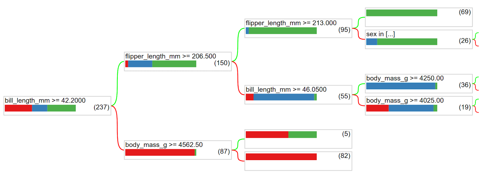
You can visually follow the tree structure. In this tree, the first decision is based on the bill length. Penguins with bills longer than 42.2mm are likely to be the blue (Gentoo) or green (Chinstrap) species, while the ones with shorter bills are likely to be of the red specy (Adelie).
For the first group, the tree then asks about the flipper length. Penguins with flippers longer than 206.5mm are likely to be of the green species (Chinstrap), while the remaining are likely to be of the blue species (Gentoo).
Model statistics are complementary additions to plots. Example statistics include:
- How many times is each feature used?
- How fast did the model train (in number of trees and time)?
- How are the nodes distributed in the tree structure (for example, what is the length of most branches?)
These and answers to more such inquiries are included in the model summary and accessible in the model inspector.
1# Print all the available information about the model2model.summary()3>> Input Features (7):4>> bill_depth_mm5>> bill_length_mm6>> body_mass_g7>> ...8>> Variable Importance:9>> 1. "bill_length_mm" 653.000000 ################10>> ...11>> Out-of-bag evaluation: accuracy:0.964602 logloss:0.10237812>> Number of trees: 30013>> Total number of nodes: 417014>> ...1516# Get feature importance as a array17model.make_inspector().variable_importances()["MEAN_DECREASE_IN_ACCURACY"]18>> [("flipper_length_mm", 0.149),19>> ("bill_length_mm", 0.096),20>> ("bill_depth_mm", 0.025),21>> ("body_mass_g", 0.018),22>> ("island", 0.012)]
In the example above, the model was trained with default hyperparameter values. This is a good first solution, but “tuning” the hyper-parameters can often further improve the quality of the model. That can be done as in the following:
1# List all the other available learning algorithms2tfdf.keras.get_all_models()3>> [tensorflow_decision_forests.keras.RandomForestModel,4>> tensorflow_decision_forests.keras.GradientBoostedTreesModel,5>> tensorflow_decision_forests.keras.CartModel]67# Display the hyper-parameters of the Gradient Boosted Trees model8? tfdf.keras.GradientBoostedTreesModel9>> A GBT (Gradient Boosted [Decision] Tree) is a set of shallow decision trees trained sequentially. Each tree is trained to predict and then "correct" for the errors of the previously trained trees (more precisely each tree predicts the gradient of the loss relative to the model output)..10 ...11 Attributes:12 num_trees: num_trees: Maximum number of decision trees. The effective number of trained trees can be smaller if early stopping is enabled. Default: 300.13 max_depth: Maximum depth of the tree. `max_depth=1` means that all trees will be roots. Negative values are ignored. Default: 6.14 ...1516# Create another model with specified hyper-parameters17model = tfdf.keras.GradientBoostedTreesModel(18 num_trees=500,19 growing_strategy="BEST_FIRST_GLOBAL",20 max_depth=8,21 split_axis="SPARSE_OBLIQUE",22 )2324# Evaluate the model25model.compile(metrics=["accuracy"])26print(model.evaluate(test_ds))27# >> 0.986851
With TensorFlow Decision Forests, you can now train state-of-the-art Decision Forests models with maximum speed and quality and with minimal effort in TensorFlow. And if you feel adventurous, you can now combine decision forests and neural networks together to create new types of hybrid models.
Conclusion
Decision trees are algorithms that are simple but intuitive, and because of this they are used a lot when trying to explain the results of a Machine Learning model. Despite being weak, they can be combined giving birth to bagging or boosting models, that are very powerful.
That is all, I hope you liked the post. Thank you very much for reading, and have a great day! 😄